The HGD Algorithm
On the uphill battle toward local minima.
Originally published on my Substack.
Once a company has a working product in production, it is incredibly difficult to make choices that might degrade it. This is a direct consequence of loss aversion1; the perceived risk of losing a customer due to a quality regression usually outweighs the potential gain of an unproven improvement.
Talking with many friends and colleagues in the AI industry in the last few months, I’ve noticed a recurring pattern that I call the HGD (Human Gradient Descent) algorithm. This is the manual, iterative process engineers and product managers use to nudge an AI agent toward a “better” state. A good example can be seen here.
What is an Agent?
Intuitively, an agent is any software with a policy: a set of rules (often probabilistic) that determines an action given a specific state. A chatbot deciding to answer you politely (action) after you ask for the time (state) is an agent. Claude Code, when it attempts to generate an entire codebase, is an agent.
Some argue an “AI agent” is specifically one where the bulk of the policy is defined by an underlying LLM. I find that definition incomplete. What constitutes “most”? Why limit it to LLMs? A more rigorous definition is this: an AI agent is any system that operates in a probabilistic environment, relying on probabilistic observations to execute a stochastic policy. (For the mathematically inclined, I’ve included a formal version of this logic at the end of the post).
The HGD Process in the Wild
How do teams actually improve their agents? Suppose a company builds an agent for automotive sales calls. The goal is simple: generate a “lead”, a case where a human customer agrees to a follow-up call from a human sales rep.
After the first version is deployed, the company begins accumulating data from real calls. Up to this point, it looks like a standard SaaS development cycle. To understand where the “agent” path diverges, we need a bit of notation. Let’s assume any conversation is a series:
\[(a_1,c_1,a_2,c_2,.....a_N,c_N)\]Where $a$ is an agent turn, $c$ is a customer turn, and the subscript is the turn number.
How should the team use this data to make the agent generate more leads? The best teams I’ve seen use a relatively simple approach - the HGD Algorithm:
-
Partition: Take a new batch of data $D$ and split it into two groups: those that generated a lead (L) and those that didn’t (NL).
-
Lock in the “Good”: For group L, create regression tests for every consecutive pair of customer-agent responses. This ensures that these “good” interactions are maintained in future versions.
-
Correct the “Bad”: For group NL, humans identify patterns describing why the agent failed. Humans then are “correcting” these patterns and adding them to the regression tests as new pairs.
Essentially, these humans are manually adding the “gradient” to the “parameters” of the model (usually the system prompt).
The Trap
It’s a simple, seductive algorithm. It even has a desirable property: it is “ever-improving.” Since every good or corrected pair becomes a regression test, you are theoretically guaranteed that the agent won’t fail on those specific examples again.
So, where is the problem? I claim this algorithm is bound to fail for three reasons:
-
Human Cognitive Limits: Humans are generally poor at inferring accurate patterns from large datasets.
-
Ignoring Compounding Errors: Conversations are processes where early actions fundamentally alter future states. If an agent makes a slightly sub-optimal choice at step 1, the distribution at step 5 is entirely different from what your regression tests expect. A well known result2 shows that the error in this case scales quadratically with the conversation length, rather than linearly.
-
Local Minima and Learning Rate Decay: This algorithm will, with high probability, get stuck in a local minima. It will never reach the performance of an optimal agent, and will likely settle very far from it. More interestingly, this process actually becomes worse as you collect more data.
While the first two points are obvious, the third is worth discussing.
The Local Minima & Learning Rate Problem
The third point is straightforward: because the algorithm is “ever-improving on every example”, you are effectively always moving “downhill” toward a lower cost (the number of “No Leads”). But what if you started your agent in a cost function that looks like this?
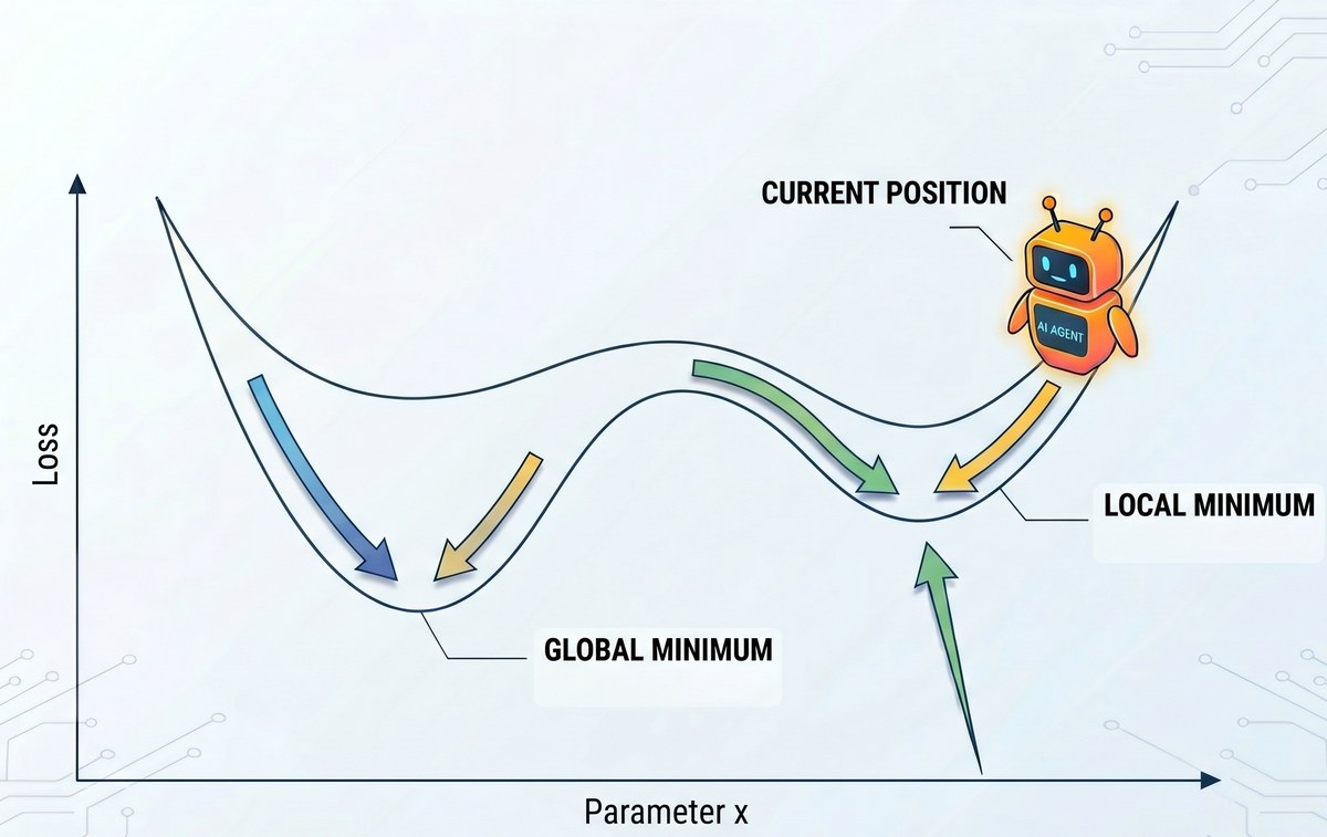
With high probability, the agent cannot escape this valley. To reach a better global minimum, the agent would likely need to “ruin” a large number of currently “good” examples to explore a better policy. Since the HGD algorithm (via regression tests) forbids any degradation, you are essentially locked into your initial, sub-optimal path. This is somewhat the opposite3 of how we would like to design systems that learn continuously, as we want the agent to learn new tasks. Moreover, the more data you add, the more regression tests you accumulate. These tests act as a massive anchor on the optimization process.
The space of allowed changes to the agent’s policy is constantly shrinking. Every new test is a new constraint. Over time, it becomes increasingly difficult for a human to find a “gradient” (a prompt change or a rule update) that actually improves the agent while passing every single existing regression test. Eventually, the “Human Gradient Descent” grinds to a halt.
Final Remarks
So, what do we do? Is there a way to fix the HGD algorithm? Let’s first define the desired qualities of any algorithm meant to substitute it:
-
Automation: It should be as human-independent as possible, ensuring efficiency in both time and cost.
-
Trajectory-Level Optimization: Unlike HGD, which optimizes myopically for isolated $(c_i, a_i)$ pairs, the solution must optimize for the entire sequence $\tau$.
-
Global Optimization: It must have the ability to find a global minimum, or at least a sufficiently deep local one.
-
Positive Scaling: Unlike HGD, it should actually improve as you collect more data, rather than grinding to a halt.
Can we satisfy these conditions?
Appendix — Mathematical Framework
Let’s define an agent more rigorously using standard Markov Decision Process (MDP) notation. Given a set of states and a set of actions:
\[\{s_i\} , \{a_i\}\]A policy is a probability distribution over the actions, given a specific state:
\[\pi(a|s)\]Now, let’s assume we have an environment—i.e., a mechanism where, given a state at time $t$ and a corresponding action $a$ by the agent, the environment has a transition function that induces a probability distribution over the next state. Mathematically:
\[P_e(s_{t+1}|s_t,a_t)\]Next, we define a trajectory. A trajectory is a sequence of states and actions, ordered in time, where each transition corresponds to either the policy or the transition function:
\[\tau=(s_0,a_0,s_1,a_1,.....s_t,a_t,......,s_T)\] \[\forall t \: P(a_t |s_t)=\pi(a_t|s_t) \;, P(s_{t+1}|s_t,a_t)=P_e(s_{t+1}|s_t,a_t)\]Optimization usually happens within the standard REINFORCE framework (where the superscript $i$ is the trajectory number, and we add a minus sign to frame it as a loss function):
\[\nabla J(\theta) \approx -\sum_{i}^N\sum_{t=0}^{T-1}\nabla \log \: \pi_\theta(a_t^i|s_t^i) \: R(\tau^i)\]So, how do we model the HGD algorithm here? We can frame it as standard gradient descent, where all the “good” examples are accumulated in every batch and assigned a high reward $G$, while new “bad” examples are added to the batch with a negative reward $B$.
To mimic the strict nature of regression testing, we assume:
\[G>0 , \; B <0, \: G\gg |B|\]What does this mean? Any trajectory contributing a reward $G$ heavily tilts the gradient in that direction, encouraging the policy to recreate this “good” trajectory. Since we force this direction to be maintained no matter what, the only gradients from the “bad” group that can actually effect change are those orthogonal to the “good” group.
However, this effectively creates a diminishing learning rate. The magnitude of the parallel direction (the “good” examples) heavily overshadows the “bad” ones. Assume we sum up these orthogonal vectors:
\[\vec{r}=B\vec{u}+G\vec{v}=G\left(\frac{B}{G}\vec{u}+\vec{v}\right)=G(\epsilon\vec{u}+\vec{v})\]When we normalize this vector to update the policy:
\[\hat{r}=\frac{(\epsilon\vec{u}+\vec{v})}{\sqrt{\epsilon^2+1}}\approx \epsilon\vec{u}+\vec{v}\]This implies that the more “good” examples (regression tests) we collect, the smaller $\epsilon$ becomes, meaning the learning rate in the orthogonal direction actively diminishes.
-
Prospect theory (Wikipedia). ↩
-
Ross, Gordon & Bagnell, A Reduction of Imitation Learning and Structured Prediction to No-Regret Online Learning (DAgger). ↩
-
Kirkpatrick et al., Overcoming Catastrophic Forgetting in Neural Networks (EWC). ↩